Basis Functions

Bspline

B-spline surfaces for freeform geometry.

B-splines are popular for describing freeform surfaces because they allow local changes to the geometry [HDKMollerA24]. Their smoothness is controlled by the spline degrees, which determine continuity and differentiability [CHB09]. A tensor-product B-spline surface is defined by two knot vectors, a grid of univariate B-spline basis functions, and a bi-directional net of control points [PT12]. Below, we summarize the main components.

Notes

Knot vectors. A surface uses two (typically clamped) nondecreasing knot vectors \(U\) and \(V\):

\[U = \{\underbrace{0,\dots,0}_{p+1},\, u_{p+1}, \dots, u_{n},\, \underbrace{1,\dots,1}_{p+1}\}, \qquad V = \{\underbrace{0,\dots,0}_{q+1},\, v_{q+1}, \dots, v_{m},\, \underbrace{1,\dots,1}_{q+1}\}.\]

Here \(p\) and \(q\) are the degrees in the \(u\)- and \(v\)-directions. A knot vector \(U=\{u_0,\dots,u_M\}\) is a nondecreasing sequence, i.e., \(u_i \le u_{i+1}\); each element is a knot.

Univariate B-spline basis (Cox–de Boor). In the \(u\)-direction (analogously for \(v\)), the basis \(\{N_{i,p}\}\) is defined recursively [PT12]:

\[\begin{split}N_{i,0}(u) = \begin{cases} 1, & u_i \le u < u_{i+1},\\ 0, & \text{otherwise}, \end{cases}\end{split}\]

\[N_{i,p}(u) = \frac{u - u_i}{u_{i+p} - u_i}\, N_{i,p-1}(u) \;+\; \frac{u_{i+p+1} - u}{u_{i+p+1} - u_{i+1}}\, N_{i+1,p-1}(u).\]

In the \(v\)-direction, the basis \(\{M_{j,q}\}\) is

\[\begin{split}M_{j,0}(v) = \begin{cases} 1, & v_j \le v < v_{j+1},\\ 0, & \text{otherwise}, \end{cases}\end{split}\]

\[M_{j,q}(v) = \frac{v - v_j}{v_{j+q} - v_j}\, M_{j,q-1}(v) \;+\; \frac{v_{j+q+1} - v}{v_{j+q+1} - v_{j+1}}\, M_{j+1,q-1}(v).\]

Control points. Control points \(\mathbf{P}_{i,j}\) link the basis to geometry. They can be scalars, 2D, or 3D vectors.

Surface definition. The tensor-product B-spline surface is

(1)\[Z(u,v) = \sum_{i=0}^{n} \sum_{j=0}^{m} N_{i,p}(u)\, M_{j,q}(v)\, \mathbf{P}_{i,j}.\]

Implementation details (this library). We use scalar control points \(\mathbf{P}_{i,j}\) (height field), uniformly increasing clamped knot vectors, and \(u,v \in [0,1]\). To couple an explicit surface to the ray tracer, we map physical coordinates \(\hat{x}_1,\hat{x}_2\) to the parametric domain via a scale \(h\):

\[S(\hat{x}_1,\hat{x}_2) = Z\!\left(\frac{\hat{x}_1}{h},\, \frac{\hat{x}_2}{h}\right).\]

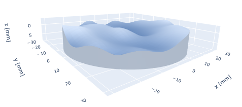
Visualization of a Freeform lens with a B-spline surface.

Examples

Define a lens with a B-spline surface and plot it:

import torch
import diffinytrace as dit

aperture_half = 30.0
aperture_radius = aperture_half
lens_thickness = 8.0
material = dit.materials["NBK7"]
transform = dit.transforms.Identity()

# degree [p, q] and control net size [n_u, n_v] (example values)
bspline = dit.Bspline(aperture_half, [3, 3], [8, 8])
plane = dit.Plane()

with torch.no_grad():
    bspline.coeff.data = torch.randn_like(bspline.coeff.data) * 3.0

lens = dit.Lens(transform, lens_thickness, bspline, plane,
                material, aperture_radius)

dit.plotting.system3D.plot(lens, zticks=[0, 5])

diffinytrace.basis_functions.bspline.cox_de_boor_recursion(U: Tensor, k: int, n: int, xis: Tensor, k_curr: int) → Tensor

Cox-de Boor recursion for B-spline basis functions.

Parameters:

• U (torch.Tensor) – Knot vector.

• k (int) – Order of the B-spline.

• n (int) – Number of control points.

• xis (torch.Tensor) – Evaluation points.

• k_curr (int) – Current recursion level.

Returns:

B-spline basis function values at the evaluation points.

Return type:

torch.Tensor

diffinytrace.basis_functions.bspline.basis_1D(points: Tensor, U: Tensor, k: int, n: int, val_range: tuple[float, float]) → Tensor

Compute 1D B-spline basis functions at given points.

Parameters:

• points (torch.Tensor) – Points where the basis functions are evaluated.

• U (torch.Tensor) – Knot vector.

• k (int) – Order of the B-spline.

• n (int) – Number of control points.

• val_range (tuple[float, float]) – Range of the target interval (e.g., (0.0, 1.0)).

Returns:

B-spline basis function values at the evaluation points.

Return type:

torch.Tensor

Raises:

RuntimeError – If the knot vector does not start at 0.0 or end at 1.0.

Example

>>> import torch
>>> import matplotlib.pyplot as plt
>>> from diffinytrace.basis_functions import bspline
>>> U = torch.tensor([0., 0.2, 0.4, 0.6, 0.8, 1])
>>> n = 3
>>> k = 3  # This is order 3
>>> print(U[0], U[-1])
>>> xis = torch.linspace(0, 1, 100)
>>> xN = bspline.basis_1D(xis, U, k, n, [0., 1.])
>>> num_points = xN.shape[0]
>>> tmp = xN.reshape(num_points, -1, 1) * xN.reshape(num_points, 1, -1)
>>> for yin in xN.T:
...     plt.plot(xis, yin)
>>> plt.gca().set_aspect('equal')

diffinytrace.basis_functions.bspline.basis_2D(points: Tensor, Us: List[Tensor], orders: List[int], ns: List[int], x_range: tuple, y_range: tuple) → Tensor

Compute the 2D B-spline basis functions for given points.

Parameters:

• points (torch.Tensor) – Points where the basis functions are evaluated.

• Us (list[torch.Tensor]) – Knot vectors for x and y directions.

• orders (list[int]) – Orders of the B-spline in x and y directions.

• ns (list[int]) – Number of control points in x and y directions.

• x_range (tuple) – Range of the target plane in the x direction.

• y_range (tuple) – Range of the target plane in the y direction.

Returns:

2D B-spline basis function values at the evaluation points.

Return type:

torch.Tensor

Example

>>> import diffinytrace as dit
>>> from diffinytrace.basis_functions.bspline import basis_2D
>>> import torch
>>>
>>> U1 = torch.tensor([0., 0.2, 0.4, 0.6, 0.8, 1])
>>> Us = [U1, U1]
>>> ps = [3, 3]
>>> ns = [3, 3]
>>>
>>> side_points = 100
>>> _x = torch.linspace(0, 1, side_points)
>>> _y = torch.linspace(0, 1, side_points)
>>> grid_y, grid_x = torch.meshgrid(_y, _x, indexing='ij')
>>> points = torch.cat([grid_x.reshape(-1, 1), grid_y.reshape(-1, 1)], dim=-1)
>>>
>>> N2D = basis_2D(points, Us, ps, ns, torch.tensor([0, 1]), torch.tensor([0, 1]))
>>>
>>> xi = 0
>>> yi = 2
>>> dit.plotting.quantity2D.plot(
>>>     N2D[:, yi, xi].reshape(side_points, side_points),
>>>     "basis fun",
>>>     [0, 1],
>>>     [0, 1],
>>>     xlabel="x",
>>>     ylabel="y"
>>> )

Raises:

RuntimeError – If the input points are not in local coordinates or have an incorrect shape.

diffinytrace.basis_functions.bspline.surface_2D(points: Tensor, Us: List[Tensor], orders: List[int], ns: List[int], x_range: tuple, y_range: tuple, control_points: Tensor) → Tensor

Evaluate a 2D B-spline surface at given points using provided knot vectors, orders, and control points.

Parameters:

• points (torch.Tensor) – Points where the surface is evaluated, shape [num_points, 2].

• Us (List[torch.Tensor]) – Knot vectors for x and y directions [U_x, U_y].

• orders (List[int]) – Orders of the B-spline in x and y directions [order_x, order_y].

• ns (List[int]) – Number of control points in x and y directions [n_x, n_y].

• x_range (tuple) – Range of the target plane in the x direction (min, max).

• y_range (tuple) – Range of the target plane in the y direction (min, max).

• control_points (torch.Tensor) – Control points, shape [n_x, n_y, …] or [n_x*n_y, …].

Returns:

Evaluated surface points at the input locations.

Return type:

torch.Tensor

Raises:

RuntimeError – If the input points are not in local coordinates or have an incorrect shape.

Example

>>> import torch
>>> from diffinytrace.basis_functions import bspline
>>> n_x, n_y = 4, 4
>>> control_points = torch.randn((n_x, n_y, 2))
>>> k_x, k_y = 3, 3
>>> U_x = torch.linspace(0, 1, n_x + k_x)
>>> U_y = torch.linspace(0, 1, n_y + k_y)
>>> points = torch.rand((100, 2))
>>> surface = bspline.surface_2D(points, [U_x, U_y], [k_x, k_y], [n_x, n_y], (0.0, 1.0), (0.0, 1.0), control_points)

diffinytrace.basis_functions.bspline.insert_knot_1D_single(U: Tensor, korder: int, new_knot: Tensor, control_points: Tensor, dim: int = 0) → Tuple[Tensor, Tensor]

Insert a single knot into a 1D B-spline knot vector and update control points.

Parameters:

• U (torch.Tensor) – Original knot vector.

• korder (int) – Order of the B-spline.

• new_knot (torch.Tensor or float) – Knot value to insert.

• control_points (torch.Tensor) – Control points (shape: [n, …]).

• dim (int, optional) – Dimension along which to insert the knot (default: 0).

Returns:

(Updated knot vector, updated control points).

Return type:

Tuple[torch.Tensor, torch.Tensor]

Example

>>> import torch
>>> import numpy as np
>>> import matplotlib.pyplot as plt
>>> n = 4
>>> control_points = torch.randn((n, 2))  # Random control points
>>> k = 4  # Quadratic B-spline
>>> U = torch.tensor([0.0] * (k - 1) + list(np.linspace(0, 1.0, n + k - 2 * (k - 1))) + [1.0] * (k - 1))
>>> U = U.float()
>>> print(U.shape[0] - k == n, n >= k)
>>> for m in range(100):
...     U_new, new_control_points = bspline.insert_knot_1D_single(U, k, torch.rand((1)), control_points)
...     print("new_control_points", new_control_points)
...     print("control_points", control_points)
...     xis = torch.linspace(0, 1, 1000)
...     xN1 = bspline.basis_1D(xis, U, k, 3, [0, 1.])
...     out1 = xN1 @ control_points
...     xN2 = bspline.basis_1D(xis, U_new, k, 4, [0, 1.])
...     out2 = xN2 @ new_control_points
...     plt.plot(out1[:, 0], out1[:, 1], linewidth=5.0)
...     plt.plot(out2[:, 0], out2[:, 1], "--")
...     torch.mean((out1 - out2) ** 2)

Chebyshev

Legendre

diffinytrace.basis_functions.legendre.precompute_legendre_polynomials(x: Tensor, degree: int) → list[Tensor]

Precomputes all Legendre polynomials up to a given degree.

Args: x (torch.Tensor): Input tensor for x-coordinates. degree (int): Maximum degree of the Legendre polynomials.

Returns: list of torch.Tensor: List of precomputed Legendre polynomials [P_0(x), P_1(x), …, P_degree(x)].

diffinytrace.basis_functions.legendre.basis_2D(points: Tensor, degree: int) → Tensor

Generates 2D Legendre polynomial basis functions up to a given degree using precomputed 1D polynomials.

Args: degree (int): Maximum degree of the Legendre polynomials. x (torch.Tensor): x-coordinates as a torch tensor. y (torch.Tensor): y-coordinates as a torch tensor.

Returns: torch.Tensor: Tensor of shape (num_basis_functions, *x.shape) with all 2D basis functions.

diffinytrace.basis_functions.legendre.get_num_coeff(degree: int) → int

Returns the number of coefficients for a given degree of Legendre polynomials. The number of coefficients is given by the formula (degree + 1) * (degree + 2) / 2.

Parameters:

degree (int) – Degree of the Legendre polynomial.

Returns:

Number of coefficients.

Return type:

int

Zernike

Zernike polynomial basis functions for optical wavefront representation.

This module provides functions to compute Zernike polynomials, which are commonly used in optics for describing wavefront aberrations over a circular aperture. The polynomials are orthogonal over the unit disk and are indexed by radial order (n) and azimuthal frequency (m).

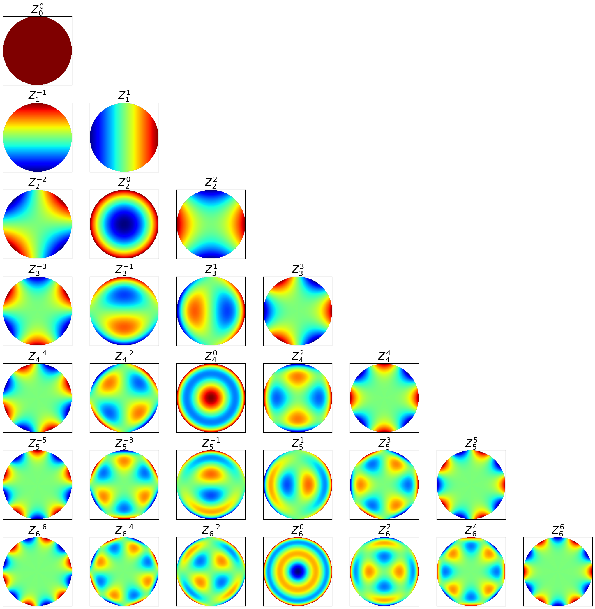
Visualization of Zernike polynomials organized by radial order (rows) and azimuthal frequency (columns).

Example

Basic usage for computing and visualizing Zernike polynomials:

>>> import torch
>>> import numpy as np
>>> import matplotlib.pyplot as plt
>>> import diffinytrace.basis_functions.zernike as zernike
>>>
>>> # Create unit circle grid
>>> grid_size = 256
>>> x = torch.linspace(-1, 1, grid_size)
>>> y = torch.linspace(-1, 1, grid_size)
>>> X, Y = torch.meshgrid(x, y, indexing='ij')
>>>
>>> # Create mask for unit circle
>>> mask = (X**2 + Y**2) <= 1.0
>>> x_points = X[mask]
>>> y_points = Y[mask]
>>> points = torch.stack([x_points, y_points], dim=1)
>>>
>>> # Evaluate Zernike polynomials
>>> max_n = 6  # Maximum radial degree
>>> basis_values = zernike.basis_function(max_n, points)
>>>
>>> # Group basis functions by radial degree
>>> basis_by_degree = {}
>>> for basis_idx in range(basis_values.shape[1]):
...     radial_order = zernike.get_radial_order(basis_idx)
...     if radial_order not in basis_by_degree:
...         basis_by_degree[radial_order] = []
...     basis_by_degree[radial_order].append(basis_idx)
>>>
>>> # Visualize the polynomials
>>> max_cols = max(len(indices) for indices in basis_by_degree.values())
>>> num_rows = len(basis_by_degree)
>>> fig, axes = plt.subplots(num_rows, max_cols, figsize=(3*max_cols, 3*num_rows))
>>>
>>> for row_idx, (radial_order, basis_indices) in enumerate(sorted(basis_by_degree.items())):
...     for col_idx, basis_idx in enumerate(basis_indices):
...         # Create 2D array with NaN outside unit circle
...         tmp = torch.full((grid_size, grid_size), float('nan'))
...         tmp[mask] = basis_values[:, basis_idx]
...
...         # Plot
...         ax = axes[row_idx, col_idx]
...         im = ax.imshow(tmp.numpy(), extent=[-1, 1, -1, 1],
...                       origin='lower', cmap='jet', vmin=-1, vmax=1)
...         azimuthal = zernike.get_azimuthal_frequency(basis_idx)
...         ax.set_title(f"$Z^{{{azimuthal}}}_{{{radial_order}}}$", fontsize=25)
...         ax.set_xticks([])
...         ax.set_yticks([])
...         ax.set_aspect('equal')
>>>
>>> plt.tight_layout()
>>> plt.show()

Notes

• Zernike polynomials are only defined for points within the unit circle (r ≤ 1)

• Radial order n determines the number of radial variations

• Azimuthal frequency m determines the angular variations and symmetry

diffinytrace.basis_functions.zernike.get_num_basis(max_radial_order: int) → int

Calculate the number of basis functions for Zernike polynomials up to a given radial order. The number of basis functions is given by the formula (n + 1) * (n + 2) / 2.

Parameters:

max_radial_order (int) – Maximum radial order.

Returns:

Number of coefficients.

Return type:

int

diffinytrace.basis_functions.zernike.get_radial_order(basis_idx: int) → int

Calculate the radial degree from the basis function index.

Parameters:

basis_idx (int) – Index of the basis function.

Returns:

Radial degree.

Return type:

int

diffinytrace.basis_functions.zernike.get_azimuthal_frequency(basis_idx: int) → int

Calculate the azimuthal frequency from the basis function index.

Parameters:

basis_idx (int) – Index of the basis function.

Returns:

Azimuthal frequency (m value).

Return type:

int

Module Contents